Area Weighted Global Temperature

imports

%matplotlib inline
import matplotlib.pyplot as plt

import xarray as xr
import numpy as np
import pandas as pd
from cartopy import crs as ccrs

from calendar import month_abbr

matplotlib parameters for the figures

plt.rcParams['figure.figsize'] = (10,8)
plt.rcParams['font.size'] = 14
plt.rcParams['lines.linewidth'] = 2

load the monthly NCEP (NCEP/NCAR) reanalysis temperature (2 m)

Downloaded from https://downloads.psl.noaa.gov/Datasets/ncep.reanalysis/Monthlies/surface/

ncep_temp = xr.open_dataset('./air.mon.mean.nc')

ncep_temp = ncep_temp.sortby('lat')

ncep_temp

selects only complete years

ncep_temp = ncep_temp.sel(time=slice(None, '2025'))

levels for plotting

levels=np.arange(-30, 30+5, 5)

levels

array([-30, -25, -20, -15, -10,  -5,   0,   5,  10,  15,  20,  25,  30])

calculate the time-averaged temperature for the 1950s and the 2010s

ncep_dec_1 =  ncep_temp.sel(time=slice('1950','1959')).mean('time')

ncep_dec_2 = ncep_temp.sel(time=slice('2010','2019')).mean('time')

parameters for the colorbar

cbar_kwargs = dict(orientation='horizontal', shrink=0.7, pad=0.05, label='\u00B0C')

map the average temperature and the difference between the 2 decades

f, axes = plt.subplots(nrows=3, figsize=(8, 14), subplot_kw=dict(projection=ccrs.PlateCarree(central_longitude=180)))

ncep_dec_1['air'].plot(ax=axes[0], transform=ccrs.PlateCarree(), levels=levels, cbar_kwargs=cbar_kwargs)

ncep_dec_2['air'].plot(ax=axes[1], transform=ccrs.PlateCarree(), levels=levels, cbar_kwargs=cbar_kwargs)

(ncep_dec_2 - ncep_dec_1)['air'].plot(ax=axes[2], transform=ccrs.PlateCarree(), levels=10, cbar_kwargs=cbar_kwargs)

[ax.set_title(title) for ax, title in zip(axes, ['1950s','2010s','difference'])]

[ax.coastlines() for ax in axes];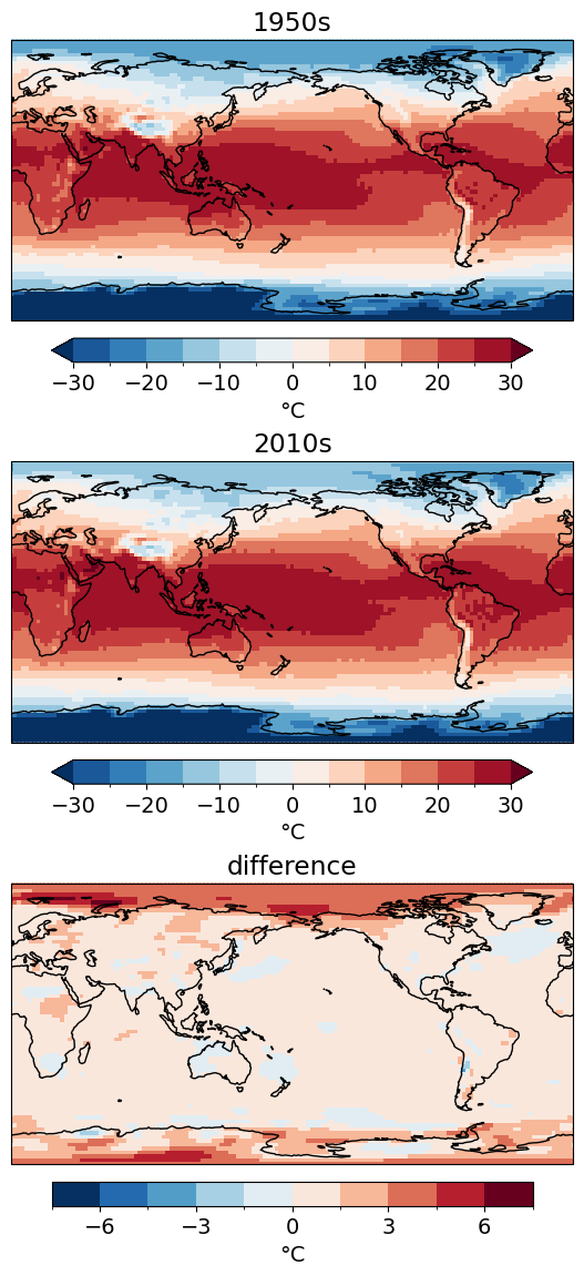

zoom in on the Northern Hemisphere high latitudes

cbar_kwargs.update(shrink=0.5)

f, axes = plt.subplots(nrows=3, figsize=(8, 14), subplot_kw=dict(projection=ccrs.NorthPolarStereo(central_longitude=0)))

ncep_dec_1['air'].plot(ax=axes[0], transform=ccrs.PlateCarree(), levels=levels, cbar_kwargs=cbar_kwargs)

ncep_dec_2['air'].plot(ax=axes[1], transform=ccrs.PlateCarree(), levels=levels, cbar_kwargs=cbar_kwargs)

(ncep_dec_2 - ncep_dec_1)['air'].plot(ax=axes[2], transform=ccrs.PlateCarree(), levels=10, cbar_kwargs=cbar_kwargs)

[ax.set_title(title) for ax, title in zip(axes, ['1950s','2010s','difference'])]

[ax.coastlines() for ax in axes]; 

[ax.set_extent([0, 360, 30, 90], crs=ccrs.PlateCarree()) for ax in axes];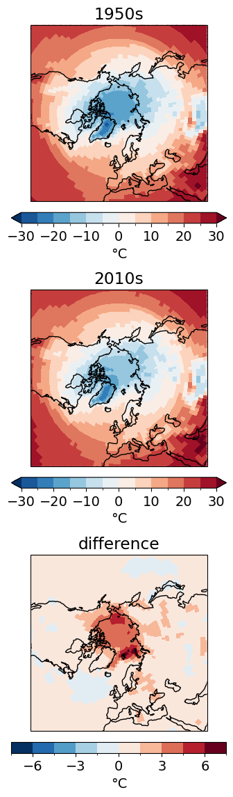

what does the time-series of surface temperature looks like for one location

Auckland_coordinates = [174.7645, -36.8509] # longitude, latitude

Auckland = ncep_temp.sel(lon=Auckland_coordinates[0], lat=Auckland_coordinates[1], method='nearest')

Auckland['air'].plot()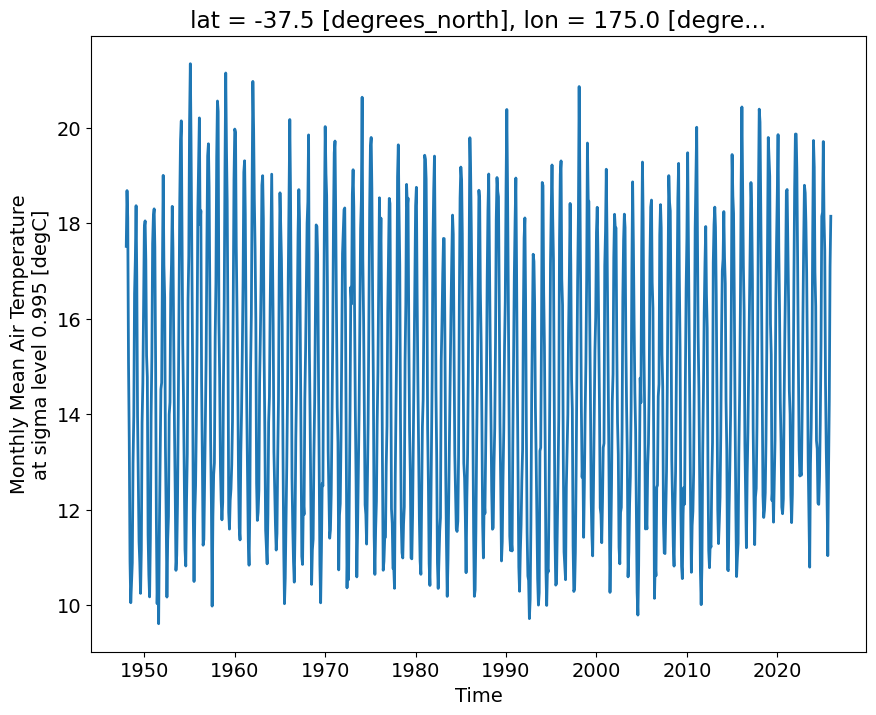

f, ax = plt.subplots()
Auckland.groupby(Auckland.time.dt.month).mean('time')['air'].plot(ax=ax, marker='o')
ax.set_xticks(np.arange(12) + 1)
ax.set_xticklabels(month_abbr[1:]); 
ax.grid(ls=':')
ax.set_ylabel('\u00B0C')

Text(0, 0.5, '°C')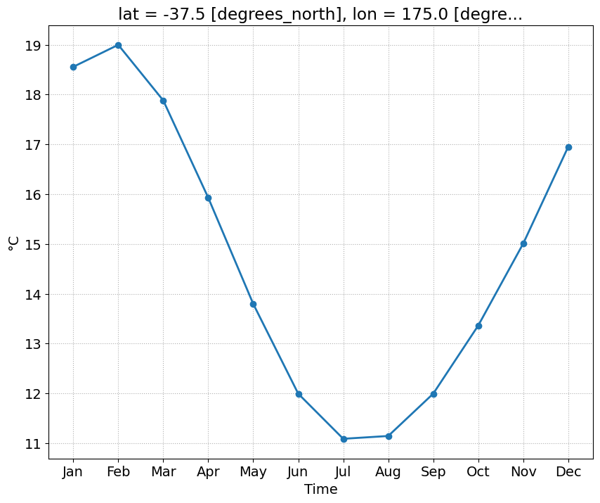

we calculate, for each grid point, the anomalies with respect to the mean seasonal cycle (average for each month)

1st step: Calculate the climatological ‘normal’ (now 1991 - 2010)

climatology = ncep_temp.sel(time=slice('1991','2010'))

climatology = climatology.groupby(climatology.time.dt.month).mean('time')

plots the climatologhy

cbar_kwargs = {'shrink':0.7, 'label':'\u00B0C'}

fg = climatology['air'].plot(figsize=(10,8), col='month', col_wrap=3, transform=ccrs.PlateCarree(), \
                            subplot_kws={"projection":ccrs.PlateCarree(central_longitude=180)}, cbar_kwargs=cbar_kwargs)

for i, ax in enumerate(fg.axs.flat):
    ax.coastlines()
    ax.gridlines()
    ax.set_title(month_abbr[i+1])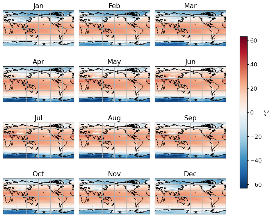

2nd step: Remove this climatology from the raw data

ncep_temp

ncep_temp_anomalies = ncep_temp.groupby(ncep_temp.time.dt.month) - climatology

plots the anomalies for the December 2025

ncep_temp_anomalies.isel(time=-1)['air'].plot()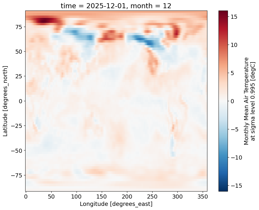

f, ax = plt.subplots(subplot_kw={"projection":ccrs.Orthographic(central_longitude=0, central_latitude=90)})
ncep_temp_anomalies.isel(time=-1)['air'].plot(ax=ax, levels=20, transform=ccrs.PlateCarree())
ax.coastlines(resolution='10m')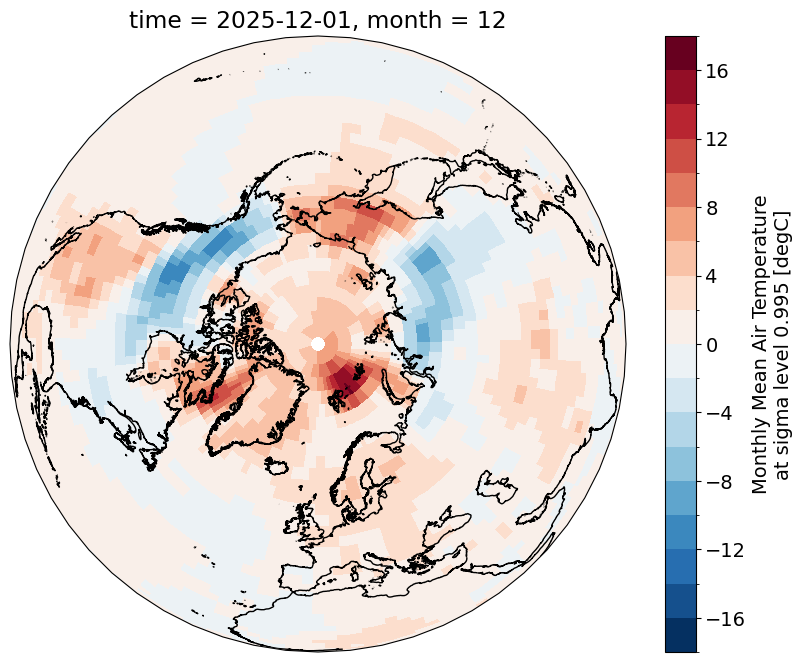

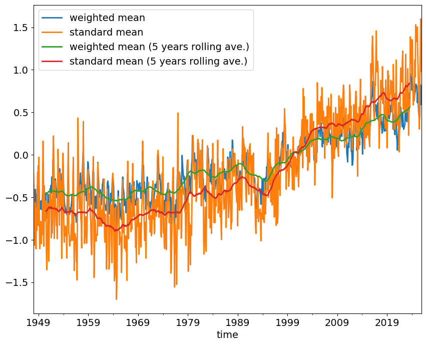
give the large difference in the area represented by grid points at low and high latitudes, we will calculate the weighted average global mean temperature anomlaies and compare the results to the standard (unweighted) anomalies

latitudes = ncep_temp['lat']

latitudes

<xarray.DataArray 'lat' (lat: 73)> Size: 292B
array([-90. , -87.5, -85. , -82.5, -80. , -77.5, -75. , -72.5, -70. , -67.5,
       -65. , -62.5, -60. , -57.5, -55. , -52.5, -50. , -47.5, -45. , -42.5,
       -40. , -37.5, -35. , -32.5, -30. , -27.5, -25. , -22.5, -20. , -17.5,
       -15. , -12.5, -10. ,  -7.5,  -5. ,  -2.5,   0. ,   2.5,   5. ,   7.5,
        10. ,  12.5,  15. ,  17.5,  20. ,  22.5,  25. ,  27.5,  30. ,  32.5,
        35. ,  37.5,  40. ,  42.5,  45. ,  47.5,  50. ,  52.5,  55. ,  57.5,
        60. ,  62.5,  65. ,  67.5,  70. ,  72.5,  75. ,  77.5,  80. ,  82.5,
        85. ,  87.5,  90. ], dtype=float32)
Coordinates:
  * lat      (lat) float32 292B -90.0 -87.5 -85.0 -82.5 ... 82.5 85.0 87.5 90.0
Attributes:
    units:          degrees_north
    actual_range:   [ 90. -90.]
    long_name:      Latitude
    standard_name:  latitude
    axis:           Y

weights = np.cos(np.deg2rad(latitudes))
weights.name = "weights"
weights

<xarray.DataArray 'weights' (lat: 73)> Size: 292B
array([-4.3711388e-08,  4.3619454e-02,  8.7155797e-02,  1.3052624e-01,
        1.7364822e-01,  2.1643965e-01,  2.5881907e-01,  3.0070582e-01,
        3.4202015e-01,  3.8268346e-01,  4.2261827e-01,  4.6174860e-01,
        4.9999997e-01,  5.3729957e-01,  5.7357645e-01,  6.0876143e-01,
        6.4278758e-01,  6.7559016e-01,  7.0710677e-01,  7.3727733e-01,
        7.6604444e-01,  7.9335332e-01,  8.1915206e-01,  8.4339142e-01,
        8.6602539e-01,  8.8701081e-01,  9.0630776e-01,  9.2387950e-01,
        9.3969262e-01,  9.5371693e-01,  9.6592581e-01,  9.7629601e-01,
        9.8480773e-01,  9.9144489e-01,  9.9619472e-01,  9.9904823e-01,
        1.0000000e+00,  9.9904823e-01,  9.9619472e-01,  9.9144489e-01,
        9.8480773e-01,  9.7629601e-01,  9.6592581e-01,  9.5371693e-01,
        9.3969262e-01,  9.2387950e-01,  9.0630776e-01,  8.8701081e-01,
        8.6602539e-01,  8.4339142e-01,  8.1915206e-01,  7.9335332e-01,
        7.6604444e-01,  7.3727733e-01,  7.0710677e-01,  6.7559016e-01,
        6.4278758e-01,  6.0876143e-01,  5.7357645e-01,  5.3729957e-01,
        4.9999997e-01,  4.6174860e-01,  4.2261827e-01,  3.8268346e-01,
        3.4202015e-01,  3.0070582e-01,  2.5881907e-01,  2.1643965e-01,
        1.7364822e-01,  1.3052624e-01,  8.7155797e-02,  4.3619454e-02,
       -4.3711388e-08], dtype=float32)
Coordinates:
  * lat      (lat) float32 292B -90.0 -87.5 -85.0 -82.5 ... 82.5 85.0 87.5 90.0
Attributes:
    units:          degrees_north
    actual_range:   [ 90. -90.]
    long_name:      Latitude
    standard_name:  latitude
    axis:           Y

xarray.DataArray

'weights'

lat: 73

-4.371e-08 0.04362 0.08716 0.1305 ... 0.08716 0.04362 -4.371e-08

array([-4.3711388e-08,  4.3619454e-02,  8.7155797e-02,  1.3052624e-01,
        1.7364822e-01,  2.1643965e-01,  2.5881907e-01,  3.0070582e-01,
        3.4202015e-01,  3.8268346e-01,  4.2261827e-01,  4.6174860e-01,
        4.9999997e-01,  5.3729957e-01,  5.7357645e-01,  6.0876143e-01,
        6.4278758e-01,  6.7559016e-01,  7.0710677e-01,  7.3727733e-01,
        7.6604444e-01,  7.9335332e-01,  8.1915206e-01,  8.4339142e-01,
        8.6602539e-01,  8.8701081e-01,  9.0630776e-01,  9.2387950e-01,
        9.3969262e-01,  9.5371693e-01,  9.6592581e-01,  9.7629601e-01,
        9.8480773e-01,  9.9144489e-01,  9.9619472e-01,  9.9904823e-01,
        1.0000000e+00,  9.9904823e-01,  9.9619472e-01,  9.9144489e-01,
        9.8480773e-01,  9.7629601e-01,  9.6592581e-01,  9.5371693e-01,
        9.3969262e-01,  9.2387950e-01,  9.0630776e-01,  8.8701081e-01,
        8.6602539e-01,  8.4339142e-01,  8.1915206e-01,  7.9335332e-01,
        7.6604444e-01,  7.3727733e-01,  7.0710677e-01,  6.7559016e-01,
        6.4278758e-01,  6.0876143e-01,  5.7357645e-01,  5.3729957e-01,
        4.9999997e-01,  4.6174860e-01,  4.2261827e-01,  3.8268346e-01,
        3.4202015e-01,  3.0070582e-01,  2.5881907e-01,  2.1643965e-01,
        1.7364822e-01,  1.3052624e-01,  8.7155797e-02,  4.3619454e-02,
       -4.3711388e-08], dtype=float32)

Coordinates: (1)

lat

(lat)

float32

-90.0 -87.5 -85.0 ... 87.5 90.0

units :: degrees_north
actual_range :: [ 90. -90.]
long_name :: Latitude
standard_name :: latitude
axis :: Y

array([-90. , -87.5, -85. , -82.5, -80. , -77.5, -75. , -72.5, -70. , -67.5,
       -65. , -62.5, -60. , -57.5, -55. , -52.5, -50. , -47.5, -45. , -42.5,
       -40. , -37.5, -35. , -32.5, -30. , -27.5, -25. , -22.5, -20. , -17.5,
       -15. , -12.5, -10. ,  -7.5,  -5. ,  -2.5,   0. ,   2.5,   5. ,   7.5,
        10. ,  12.5,  15. ,  17.5,  20. ,  22.5,  25. ,  27.5,  30. ,  32.5,
        35. ,  37.5,  40. ,  42.5,  45. ,  47.5,  50. ,  52.5,  55. ,  57.5,
        60. ,  62.5,  65. ,  67.5,  70. ,  72.5,  75. ,  77.5,  80. ,  82.5,
        85. ,  87.5,  90. ], dtype=float32)

Attributes: (5)
units :
degrees_north
actual_range :
[ 90. -90.]
long_name :
Latitude
standard_name :
latitude
axis :
Y

weights.plot()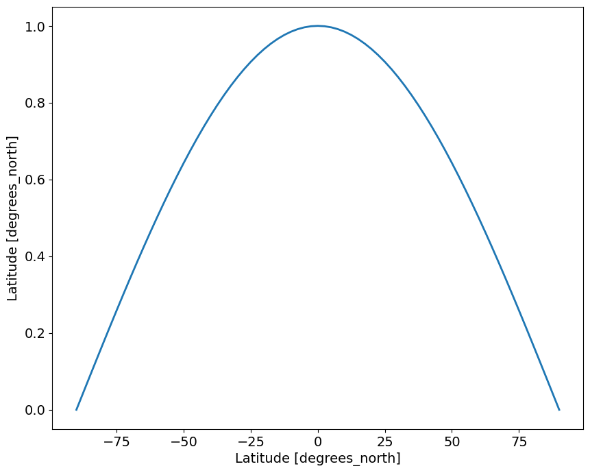

Standard mean

standard_mean = ncep_temp_anomalies['air'].mean(['lat','lon'])

standard_mean_smooth = standard_mean.rolling(time=12*5, center=True).mean().dropna("time")

Weighted mean

weighted_mean = ncep_temp_anomalies['air'].weighted(weights)

weighted_mean = weighted_mean.mean(("lon", "lat"))

weighted_mean_smooth = weighted_mean.rolling(time=12*5, center=True).mean().dropna("time")

fig, ax = plt.subplots()
weighted_mean.plot(ax=ax, label='weighted mean', color='coral', lw=0.5, alpha=0.5)
standard_mean.plot(ax=ax, label='standard mean', color='steelblue', lw=0.5, alpha=0.5)
weighted_mean_smooth.plot(ax=ax, label='weighted mean (5 years rolling ave.)', color='r')
standard_mean_smooth.plot(ax=ax, label='standard mean (5 years rolling ave.)', color='b')
ax.legend(fontsize=12, frameon=False)
ax.grid(ls=':')
ax.axhline(0, color='k', zorder=0)
ax.set_title('NCEP/NCAR global temperature average')
ax.set_ylabel('\u00B0C' + ' anomaly')

Text(0, 0.5, '°C anomaly')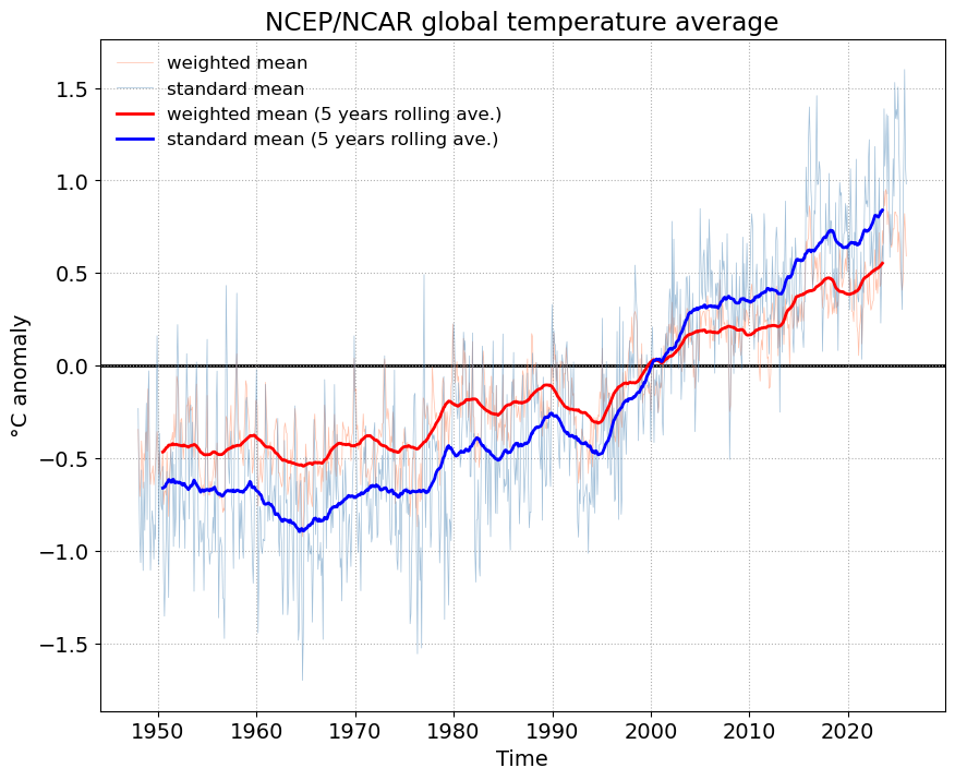

exporting the time-series in csv

weighted_mean.name = 'weighted mean'

standard_mean.name = 'standard mean'

global_means = xr.merge([weighted_mean, standard_mean])

global_means = global_means.to_pandas()

global_means.head()

	month	weighted mean	standard mean
time
1948-01-01	1	-0.344417	-0.231683
1948-02-01	2	-0.533902	-0.662671
1948-03-01	3	-0.706991	-0.923734
1948-04-01	4	-0.618840	-1.064454
1948-05-01	5	-0.407124	-0.564210

global_means = global_means.drop('month', axis=1)

global_means.head()

	weighted mean	standard mean
time
1948-01-01	-0.344417	-0.231683
1948-02-01	-0.533902	-0.662671
1948-03-01	-0.706991	-0.923734
1948-04-01	-0.618840	-1.064454
1948-05-01	-0.407124	-0.564210

global_means.plot()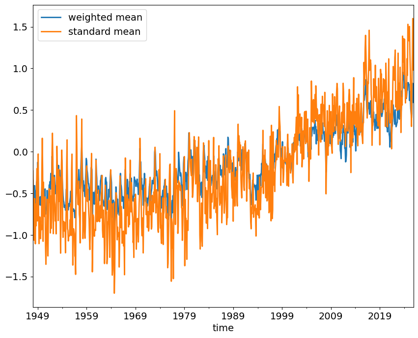

global_means_smooth = global_means.rolling(window=12*5, min_periods=12*5, center=True).mean()

global_means_smooth.columns = ['weighted mean (5 years rolling ave.)', \
                               'standard mean (5 years rolling ave.)']

global_means_smooth.plot()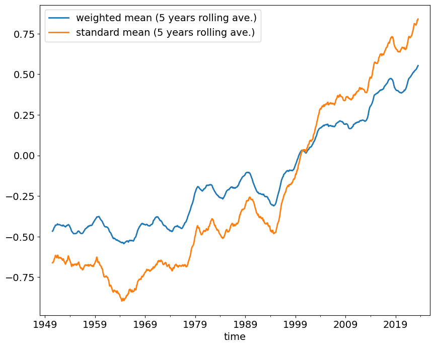

all_means = pd.concat([global_means, global_means_smooth], axis=1)

all_means

	weighted mean	standard mean	weighted mean (5 years rolling ave.)	standard mean (5 years rolling ave.)
time
1948-01-01	-0.344417	-0.231683	NaN	NaN
1948-02-01	-0.533902	-0.662671	NaN	NaN
1948-03-01	-0.706991	-0.923734	NaN	NaN
1948-04-01	-0.618840	-1.064454	NaN	NaN
1948-05-01	-0.407124	-0.564210	NaN	NaN
...	...	...	...	...
2025-08-01	0.455712	0.771791	NaN	NaN
2025-09-01	0.726205	1.156209	NaN	NaN
2025-10-01	0.821570	1.600003	NaN	NaN
2025-11-01	0.708482	1.075574	NaN	NaN
2025-12-01	0.591523	0.981019	NaN	NaN

936 rows × 4 columns

all_means.to_csv('./NCEP_global_means.csv')

data = pd.read_csv('./NCEP_global_means.csv', index_col=0, parse_dates=True)

data.head()

	weighted mean	standard mean	weighted mean (5 years rolling ave.)	standard mean (5 years rolling ave.)
time
1948-01-01	-0.344417	-0.231683	NaN	NaN
1948-02-01	-0.533902	-0.662671	NaN	NaN
1948-03-01	-0.706991	-0.923734	NaN	NaN
1948-04-01	-0.618839	-1.064454	NaN	NaN
1948-05-01	-0.407124	-0.564210	NaN	NaN

data.plot()